This document provides a reproducible text analysis of the Man the Hunter volume (Lee & DeVore, 1968) in particular to assess a word cloud presented in Venkataraman et al. (2026). It demonstrates that the word cloud presented in that paper inadvertently suppressed the word “man” through use of a default stopword list (onix) that treats “man” and “men” as generic terms for “human” while retaining “woman” as a content word. It also examines the relative frequency with which hunting and gathering (and men and women) are discussed in the volume, and the contexts in which these terms appear.
Data and Methods
The text of Man the Hunter (Lee & DeVore, 1968) was obtained from the Internet Archive (plain text format). Analysis was conducted in R using the tidytext, textstem, and wordcloud packages. The table below summarizes the key methodological choices.
Show code
tibble(Step =c("Source text", "Lines included", "Lemmatizer","Stopword lists", "Minimum word length"),Detail =c("Internet Archive djvu.txt (Man the Hunter, Lee & DeVore 1968)","Lines 746 to 36,991 (main text only, excluding front matter and references)","textstem R package (dictionary-based lemmatization)","tidytext stop_words: SMART, Snowball, onix","3 characters" )) %>% knitr::kable()
Step
Detail
Source text
Internet Archive djvu.txt (Man the Hunter, Lee & DeVore 1968)
Lines included
Lines 746 to 36,991 (main text only, excluding front matter and references)
Lemmatizer
textstem R package (dictionary-based lemmatization)
Stopword lists
tidytext stop_words: SMART, Snowball, onix
Minimum word length
3 characters
Loading and Processing the Text
The raw text file is downloaded once and cached locally. The following cleaning steps are applied before analysis:
Apostrophe variants (curly quotes, backticks) are standardized to a straight apostrophe
Windows-style line endings are converted to Unix style
Words split across lines with a hyphen are rejoined (e.g., anthro-\npologists becomes anthropologists)
Standalone page numbers are removed
The compound huntergatherer, created by the line-break joining step, is split back into two tokens
Show code
if (!file.exists("MtH.txt")) {download.file("https://ia801705.us.archive.org/30/items/ManTheHunter/Man%20the%20Hunter_djvu.txt",destfile ="MtH.txt" )}mth_unmodified <-readLines("MtH.txt")# Line number limits for the main text in the filepreface_starts <-75# start of the prefac (not used)part1_starts <-746# start of main text (after front matter)references_starts <-36991# end of main text (before references)raw <- mth_unmodified[part1_starts:references_starts]modified_text <-paste(raw, collapse ="\n") %>%gsub("['\u2018\u2019\u201A\u201B\u0060\u00B4]", "'", .) %>%# standardize apostrophesgsub("\r\n", "\n", .) %>%# fix line endingsgsub("([a-z])-\\s*\n\\s*([a-z])", "\\1\\2", .) %>%# rejoin hyphenated linebreaksgsub("(?m)^\\s*\\d+\\s*$", "", ., perl =TRUE) %>%# remove page numbersgsub("huntergatherers?\\b", "hunter gatherer", .) %>%# split inaccurate compoundgsub("huntinggathering", "hunting gathering", .) # split inaccurate compound
Tokenizing and Lemmatization
Tokenization splits the text into individual words. Lemmatization then reduces each word to its root form; for example, “cats” becomes “cat” and “running” becomes “run”. Notably, the lemmatizer correctly distinguishes between hunt (the verb) and hunter (the noun), keeping them as separate tokens. Possessive suffixes ('s) are stripped before lemmatization since the lemmatizer does not handle them consistently.
Stopwords are common words removed before analysis, typically function words like “is”, “the”, “and”. The tidytext package bundles three English stopword lists: SMART, Snowball, and onix. When used together (the default), any word appearing in any of the three lists is removed.
The onix stopword list is and older and larger list designed for search indexing. As such, it contains “men” and “man” but not “woman” or “women.” As the Appendix below shows, this is rare for an English stop word list and is likely the result of its age and original context.
full_sum_table <- bag_of_words %>%count(word, sort =TRUE) %>%mutate(orig = word %in% base_stopwords$word,no_onix = word %in% no_onix_stopwords$word,man_back = word %in% cut_stopwords$word ) %>%filter(!orig |!no_onix |!man_back)
In this case, using the onix list inadvertently removes a semantically significant word, and part of the title, from the analysis. Three versions of the stopword list are used here for comparison:
Using the default tidytext list of all three.
Using the default list , but manually removing “man” and “men”
Excluding the onix list entirely
Word Clouds
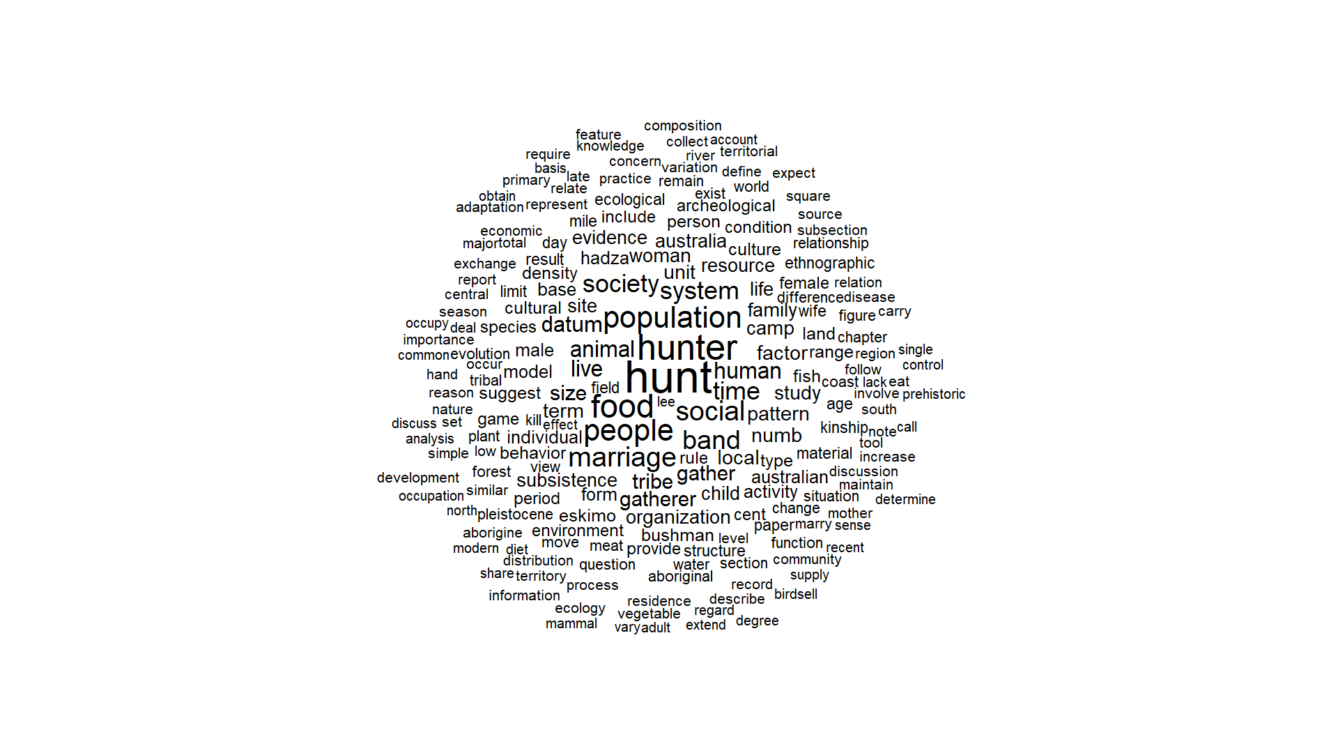
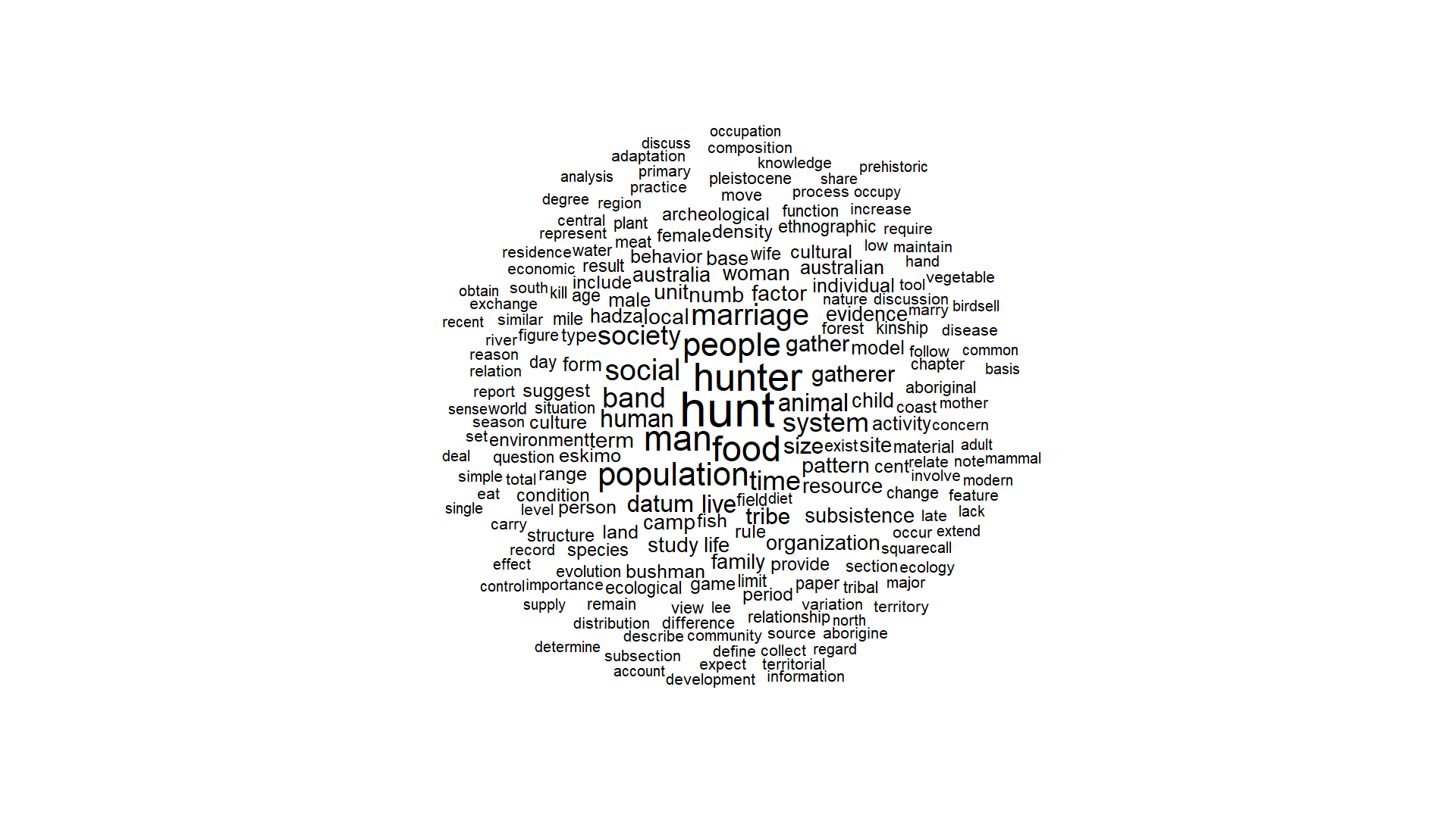
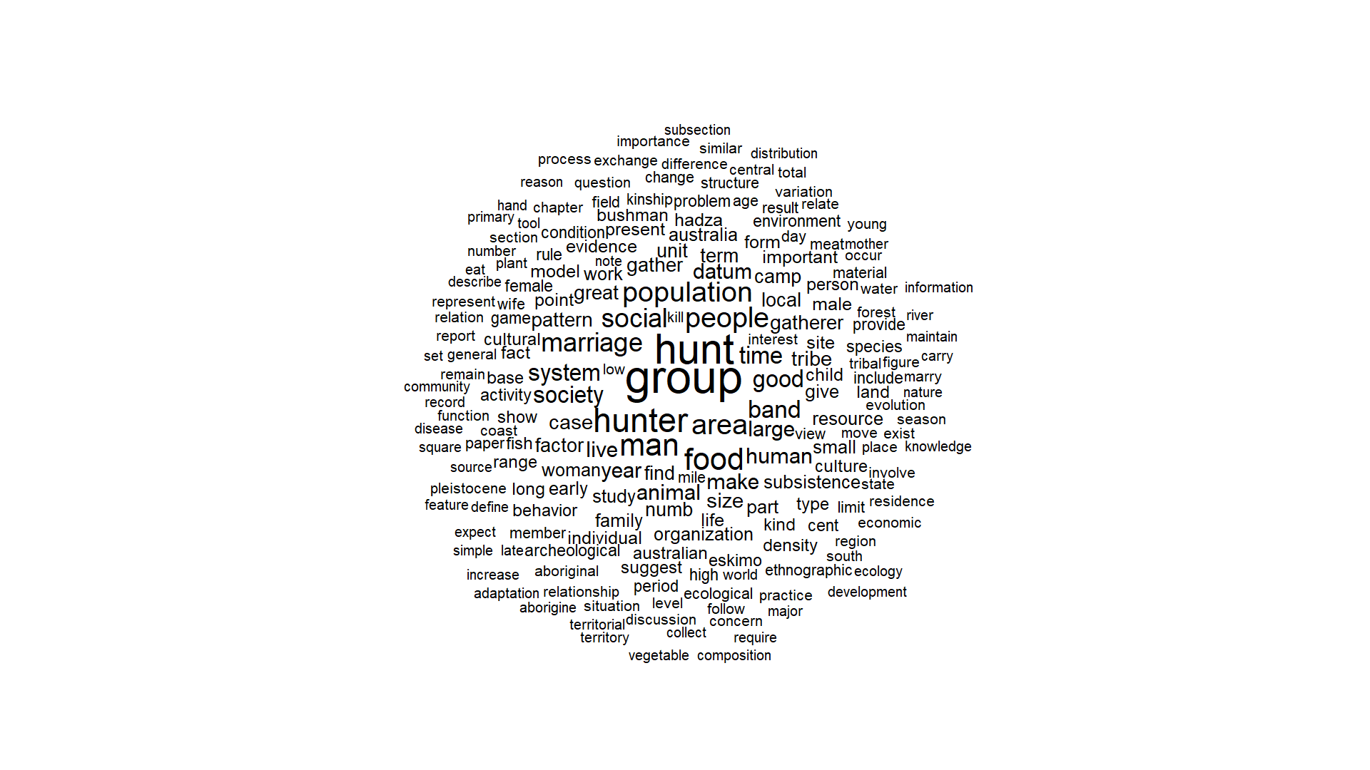
The word clouds below replicate the style of Figure 3 in Venkataraman et al. (2026), with word size proportional to frequency. Three versions are shown, one for each stopword configuration. Each cloud is followed by a table of the 10 most frequent words in that version.
Word cloud with default stopword list applied; ‘man’ and ‘men’ are absent.
The 10 most frequent words using the default stopword list are shown below. Venkataraman et al. (2026) report approximately 835 occurrences of “hunt” in their Figure 3; our replication yields 883 occurrences. The small discrepancy likely reflects minor differences in text extraction or preprocessing between the two analyses.
Show code
top10_table(full_sum_table, orig)
Word
Frequency
hunt
883
hunter
655
food
563
people
504
population
496
social
446
marriage
434
band
401
time
370
system
368
2. With “man” and “men” restored
Identical to above, but with “man” and “men” removed from the stopword list (so included in the final product).
Word cloud with the onix stopword list excluded. Additional contextually meaningful words become visible, including ‘group’, the most frequent word in the volume.
With the onix list excluded, “group” emerges as the most frequent word, a term with clear contextual relevance to a volume about human social organisation. The top 10 words are:
Show code
top10_table(full_sum_table, no_onix)
Word
Frequency
group
1014
hunt
883
hunter
655
man
568
food
563
area
509
people
504
population
496
social
446
marriage
434
Words removed by the onix list with more than 50 occurrences
The following words were suppressed in the original word cloud by the onix stopword list despite appearing more than 50 times in the main text. Some are genuine function words, but many (including “group”, “man”, “member”, and “area”) carry substantive contextual meaning in an analysis of hunter-gatherer social organisation.
Show code
onix_removed <- full_sum_table %>%filter(n >50) %>%filter(!no_onix & orig) %>%select(word, n) %>%arrange(desc(n))n_onix_removed <-nrow(onix_removed)dt_table(onix_removed,caption =paste(n_onix_removed, "words suppressed by the onix stopword list with more than 50 occurrences."),pageLength =10)
Gender and Subsistence Term Frequencies
It has also been argued that the Man the Hunter volume was broader than commonly portrayed and gave meaningful attention to women’s contributions to subsistence. The raw frequencies of key terms can help address this directly.
Hunt/hunting is mentioned 3 times as often as gather/gathering (1538 vs. 519) and man/men is mentioned 2.6 times as often as woman/women (568 vs. 220).
Contextual Analysis: Hunter-Gatherer as a Compound
The frequencies above require an important qualification. “Hunter-gatherer” is a compound term used throughout the volume, and the tokenization process splits it into two separate tokens. This inflates the apparent frequency of both “hunter” and “gatherer” relative to their independent usage. The analysis below examines how often each term appears alongside the other.
Approximately 70.5% of the 526 occurrences of “gather” are immediately preceded by “hunt”, confirming that the majority of gather/gatherer instances are part of the compound “hunter-gatherer” rather than independent references to gathering as a subsistence activity. By contrast, hunt/hunting is followed by a gather variant in approximately 24% of cases, meaning around three quarters of hunting references stand independently of the compound. The most common word preceding “hunt” is “man”, accounting for 2.4% of occurrences.
Appendix: Survey of Stopword Lists
To assess how unusual it is for a stopword list to contain “man” or “men”, we examined 68 English stopword lists compiled by igorbrigadir/stopwords, a comprehensive repository of stopword lists from NLP tools, search engines, and text analysis libraries.
Show code
if (!dir.exists("stopwords-master")) {download.file("https://github.com/igorbrigadir/stopwords/archive/refs/heads/master.zip",destfile ="stopwords-master.zip" )unzip("stopwords-master.zip")}sw_files <-list.files("stopwords-master/en/", pattern ="\\.txt$",full.names =TRUE)sw_results <-map_df(sw_files, function(f) { words <-readLines(f, warn =FALSE) %>%tolower() %>%trimws()tibble(file =basename(f),n_words =length(words),has_man ="man"%in% words,has_men ="men"%in% words,has_woman ="woman"%in% words,has_women ="women"%in% words )}) %>%left_join(sw_details <-read_csv("stopwords-master/en_stopwords.csv"), by ="file" )n_lists <-nrow(sw_results)n_with_man <-sum(sw_results$has_man)
Frequency of gendered terms across 68 English stopword lists.
Term
Lists containing term
Total lists
Percent
man
4
68
5.9
men
3
68
4.4
woman
0
68
0.0
women
0
68
0.0
No stopword list contains “woman” or “women”. 4 lists contain “man” and r``sum(sw_results$has_men) contain “men”. These 4 can be seen below. Of them, several seem to have been based on the onix list.
The onix list was developed by Lextek International in the early 1990s as part of a commercial text retrieval toolkit. Its inclusion of “man” reflects an assumption common in information retrieval of that era: that “man” usually functions as a generic synonym for “human” and is thus uninformative as a search term, while “woman” is a specific context word. This assumption is an example of the inherent bias and ambiguity in English, but also serves as a reminder that careful reading of stopword lists should be a part of any textual analysis.